Inheriting a spreadsheet from someone else

There will be times when you have to work with a spreadsheet which someone else created. It might have various issues – it might not work properly, it might be appalling to use, the formulae might be wrong – all sorts of reasons why you might end up just thinking it’s better to redesign it.

If this is the case for you, please read on.

First steps:

• Do a Save As, or otherwise create a copy. Do NOT run the risk of overwriting the original in case you need to refer back to it!
• Use Ctrl + Home, Ctrl + End and Ctrl + arrow keys to look across the whole data, so you get a sense of what it is you’re looking at.
• Unhide all columns and rows in case any are hidden.
• Widen all columns and rows, to see everything clearly.
• Check for blank rows and columns. Don’t delete too readily; they may be there for a reason. Only delete them if you are genuinely sure they should not be there.
• Run a spell check.
• Use Find & Replace to correct any repeated errors (such as . instead of / in dates).
• Consider removing formatting if it is hindering you inspecting the spreadsheet. You can do this easily via Home, Clear (on the far right of the Home tab), Clear Formats – but please be careful not to choose Clear All, which literally deletes everything. Remember, though, that dates will resort back to ‘serial numbers’, which can be very disconcerting.
• Go to Home, Find & Select (on the far right of the Home tab), Formulas. Now, apply colour to all cells which have been highlighted. Go through all the formulae to ensure that not only are they consistent, but that you understand what they do. Repeat Home, Find & Select, Formulas and remove the colouring afterwards, if you need.

Redesigning

• If it’s just too unwieldy to work with in its current state, feel free to start from scratch, taking care to consider time wasted in redesigning offset against time saved in an improved version (your manager will thank you).
• Build back into the spreadsheet any aspects of functionality which will improve use, such as Freeze Panes, formulae at the top, a Notes column at the end, colour coding, and everything else covered in Spreadsheet Design and Data Integrity.

Good spreadsheets…

• always have column headings
• never have completely blank rows or columns
• have appropriately formatted data
• are designed with the user in mind.

Even better spreadsheets…

• include a key or notes to explain aspects if needed
• have some kind of unique reference for each line, if appropriate, to aid data checking or looking things up
• use features like Freeze Panes if it helps
• have the formula(e) placed at the top if the data is going to keep growing
• NEVER have a value in a formula.

Happy spreadsheeting!

As this was an additional post with nothing to do with the exam, you might want to just click your Back button & carry on with your learning. Or, you can return to the Data Integrity or Spreadsheet Design pages.

Additional logical functions

These are NOT part of the AAT synoptic, but I deem them sufficiently useful that it warrants going over them – particularly how to hide an error message. However, if you only want to learn what you need for the exam and no more, then click here to continue.

If you’re curious, then please, dear reader, come follow… caution: mind-altering formulae ahead!

Hiding error messages with IFERROR

This is a fantastically useful function. I use it a lot for spreadsheets I’m designing for others to use. Basically, it hides error messages (anything that starts #, like #N/A or #DIV/0!) so your users don’t get freaked out – and of course there’s always the thing that it looks kind of neater too.

Consider this example here, where having entered a name which isn’t on the list, my VLOOKUP has returned a #N/A in cell B2. It would be very useful to be able to say something like ‘no-one of that name’ or even not show anything at all.

What we need to do is use the IFERROR function. Let’s have a look at it.

=IFERROR ( value , value_if_error )

It seems simple enough – only two arguments – but it can confuse people a little bit. What it’s saying is If that’s an error, do this instead. We can work through it like this: The first argument, value, is the formula that’s generating the error. That’s right, the formula in its entirety is going to be our first argument. The second argument, value_if_error, is what we want to happen if indeed there is an error – have a useful message or maybe not show anything at all.

That will mean my function will look like:

=IFERROR ( VLOOKUP(B1,A5:B9,2,0) ,“no-one of that name” )

Now I needn’t worry about the #N/A as it’s all taken care of.

The IS functions

There are nine functions in the IS group, and they all return TRUE or FALSE. They are most commonly used to check for errors in data entry or as the result of formulae. For instance, if cell A1 appeared to have a numeric value in it, you could check by saying =ISNUMBER(A1). If A1 is a number, it would return TRUE. If it wasn’t, it would return FALSE.

You can harness these by having them as your first argument in an IF statement. Supposing you want to multiply cell B2 by the VAT rate, 20%. However, that’s going to fail if someone puts a text value in B2, instead of a numeric value. So, we could say:

=IF ( ISNUMBER (B2) , B2*20% , “please enter a number“)
If it’s true that B2 is numeric then multiply it by 20%, otherwise display the text “please enter a number”.

The complete family of IS functions comprise ISBLANK, ISERR, ISERROR, ISLOGICAL, ISNA, ISNONTEXT, ISNUMBER, ISREF, and ISTEXT.

– ISNA and ISREF test specifically for the presence of #N/A and #REF errors respectively.
– ISERROR tests for an error – any error.
– ISERR tests for any error but #N/A.

AND and OR

Here are a couple of functions which can totally blow your IF statement wide open. These two functions are really simple and hugely widen the scope of an IF.

• AND looks at various conditions and if ALL are true, returns TRUE. If just a single condition is not true, it returns FALSE.

In the example below, all my conditions are that the three values are above 30. All of them are; so we have an answer of TRUE.

In this example, one of my conditions is now below 30. This causes AND to return FALSE.

• OR looks at various conditions and if just ONE is true, returns TRUE. If no conditions are true, it returns FALSE.

In the example below, my conditions are that the three values are above 30. Even though one of them isn’t, it doesn’t matter – at least one of them is so we have an answer of TRUE.

In this example, none of my conditions is now above 30. This causes OR to return FALSE.

• How do we use these? We nest them as the first argument of an IF (logical_test). As an example, supposing in a qualification you only get a certificate if you pass five exams, not just one? We would need an AND in order to test that all cells concerned have values above 70.

In the first example here, our candidate failed Exam 5, so doesn’t get a certificate:

Our second candidate has passed all five, so we can award them their certificate.

Note how the whole of the logical_test is the AND function:

Exciting formula ahead!

So… you’re wondering what you’d do if you had to go off the Result, not the Score? This calls for a bit of a stop-and-think…. I need to check:

• that C2 says either “distinction, “merit” or “pass” AND
• that C3 says either “distinction, “merit” or “pass” AND
• that C4 says either “distinction, “merit” or “pass” AND
• C5 AND C6 etc….

so I need ORs and an AND. And I need my ORs inside – nested in – my AND. Check this out. This is fun!

=IF(AND(OR(C2="distinction",C2="merit",C2="pass"),OR(C3="distinction",C3="merit",C3="pass"),OR(C4="distinction",C4="merit",C4="pass"),OR(C5="distinction",C5="merit",C5="pass"),OR(C6="distinction",C6="merit",C6="pass")),"Award certificate","no certificate")

Break it down. Look at it carefully. Count the open and close brackets – a pair each for each OR, a pair for the AND, a pair for the IF. Count the commas – one to separate each OR in the AND, one to separate the AND from the other two arguments of the IF. I’m certain you’ll find that if you’re really careful, you actually can follow the logic of what’s going on. I’ve coloured the different arguments here so you can see more easily what’s happening.

Wow, right? How cool is that? And it’s *mind-blowing* that you can work your way through it and create something like this yourself!

It really is a case of looking at what’s going on with a critical, careful eye and working your way logically through the symbols. After all, at this point, you know that any time you see Word( you know you’re looking at a function. You can have a look at the Help files in Excel and understand a lot more of what it’s explaining about that function – you know what syntax, arguments, cells, values, ranges and so on are. You understand the $ and the “double quotes”. There are only a couple of other symbols you should learn (covered in this post) and you can genuinely look at anything anyone has created and work out what’s going on.

I appreciate I went way off-piste on this, in terms of what you need for the synoptic, but I hope you now appreciate why I wanted to go through this. The power of all these functions combined is truly, truly staggering – and you have the key to it all. Enjoy!

Have a play

Please feel free to download some exercises here – lots of worksheets for you to get your teeth into. If you’re feeling brave, recreate the nested IF/AND/OR above!

If you’re following the suggested Learning Plan, please click here to go to the next post.

Combining formulae and functions

Using the formulae and functions we’ve covered thus far will enable you to really do some quite fab things, but when you harness two or more together, the sky’s the limit. It’s really quite exciting when you realise how you can do this, not only in terms of pushing your spreadsheets’ usefulness way forward but also in terms of getting that feel-good factor from achieving something really quite complicated you didn’t think you’d be able to do!

By the way, having viewed this on several screens, sometimes the animated gifs work really well and on other devices they’re really bad. So please download the associated PowerPoint file where all the animations can be viewed a lot more readily. Remember to download otherwise it won’t animate.

Two or more formulae in a single cell

The first type of combination formulae is one which eludes people new to the concept, but which is also kind of obvious when you think about it. You have to be quite nimble with the grey matter to start off with!

Remember way back when we first started looking at functions, we had an exercise called StationeryOrder? This asked us to calculate the cost, the VAT and the total cost of each line. As part of the exercise, I asked you to consider how you could create a single formula which would do all three operations in one.

Below, I’ve set out the start of the problem:

Now, in our column called Combined, we need to end up with the value 21.6, as that’s the answer. How do we get there? With these kinds of formulae you need to break the problem down. It’s easier to work in small steps, and build up as you go.

Step 1: break down the problem

• The first step was to multiply 100 by 0.18 – that gave us the Net: 18.
• Then we multiplied that by 20% to get the VAT: 3.6.
• Then we added it together to get the gross: 21.6.

Step 2: convert to actual numbers

I also often ‘convert’ what I’m doing into the actual numbers, then once I’ve got something which works I will replace them with the cell references. It often helps to use ‘real numbers’. So here, rather than worry about where my 100 is, I shall just think of 100.

In this particular example, the stumbling block for many is the fact that our middle part – VAT – comes off the back of our first part. But supposing we didn’t have that? We’d have to type 100 * 0.18 * 20%.

So if our first part is 100 * 0.18 and our second part is 100 * 0.18 * 20% then basically we’re going to add the two parts together 100 * 0.18 + 100 * 0.18 * 20%. Let’s try that.

Awesome, I get the same answer! I know I’m doing something right, now!

Incidentally, if I wanted to, I could have used brackets to ‘isolate’ each chunk, which might make it visually easier to read. =(100 * 0.18) + (100 * 0.18 * 20%). Remember BIDMAS? The multiplication would happen first anyway, so in this instance it doesn’t really matter – but there’s nothing to stop you putting them in if it helps you!

Step 3: Switch back to cell references

Now we’ve worked out which combination of the numbers actually works, it’s just a case of switching out and replacing them with the cell references.

By the way, sometimes I do this on paper and literally cross out the numbers and write the cell refs. Then I type it up. How you do this is down to you!

You’ll note my final check was to see if the answers in the combined formula (column H) matched the answer from the formula created in steps (columns D to F). They do, so that’s a great guarantee you got it right!

A formula and a function

It’s not just a case of having two formulae working together in a single cell. You could also have a function with a formula.

In this example, we’re using the principles in IAS2, that is, we always value inventory at the lower of Cost or Net Realisable Value. Once we’ve done that, we need to work out the total value of each inventory line.

Step 1: break down the problem

• First of all we have to calculate our NRV by subtracting the costs of sale from the selling price.
• Then we have to ascertain which is lower, the Cost or the NRV. This can be done with a MIN function.
• Finally we have to multiply the answer by the quantity of items we have in stock.

Obviously, we need to have column F to set out the NRV separately, but we could combine what’s going on in columns G and H into a single formula.

Step 2: convert to actual numbers

Our first answer is £12.50 because that’s the lower of the cost and NRV. Then we’re multiplying by 180.

So we need to type =12.50*180.

Step 3: Switch back to cell references

12.50 was done by the MIN, and 180 is in cell B2. So, we could type =MIN (C2, F2) * B2.

Quick check to see my combined function/formula matches the step-by-step formula – it does – and I’m good to go.

A function within a function

The last type of combination formula is the sort where you actually tuck a formula or a function inside a function (instead of them being ‘side by side’ like above).

Take this example here. I want to give a bonus of 35% if the total sales for each assistant is greater than £90.

Step 1: break down the problem

If I give a bonus only when it’s over £90, that’s an IF statement. But how will I work out the total of each sales assistant? That would be a SUMIF.

I need to say “if the total is greater than 90, multiply the total by a bonus percentage, otherwise give nothing”.

Let’s break that down into two separate columns:

• SUMIF will give us Aishah’s total sales.
• IF will decide if she gets a bonus.

Remember, I’ll need to absolute some of these cell and range references to enable me to Autofill my formula down.

Step 2: convert to actual numbers/words

Here we’re thinking If Aishah’s sales are greater than 90, then multiply Aishah’s sales by 35%, otherwise give her nothing.

Wherever it says Aishah’s sales, that’s your SUMIF. And the whole thing is the IF.

So it looks like we’ll have two SUMIFs in the one IF! Brace yourself, this often blows people’s minds!

Step 3: Switch back to cell references

We already have the following:

• = SUMIF ( $A$2:$A$12 , D3 , $B$2:$B$12 )
• = IF ( E3 > 90 , E3 * $E$1 , 0 )

In the IF, each E3 is Aishah’s total, so each E3 is where my SUMIF needs to go. So let’s put that SUMIF into the mix!

= IF ( SUMIF ( $A$2:$A$12 , D3 , $B$2:$B$12 ) > 90 , SUMIF ( $A$2:$A$12 , D3 , $B$2:$B$12 ) * $E$1 , 0 )

Can you see how we’ve literally taken the whole SUMIF – brackets and everything – and slotted it straight into the IF? Let’s see it in action:

I cheated and copied the entirety of the SUMIF – without the = at the start – as I knew I’d be needing it twice. So for the second one, I just pasted it in, rather than typing it all out afresh. In order to do this, I used the keyboard shortcuts Ctrl+C for Copy and Ctrl+V for Paste.

If you look carefully, you can see the main opening and closing brackets (parentheses) of the IF are black, and the opening and closing brackets of the SUMIF are red:

This pairing of brackets can be really handy.

How to do this for real

As they’re fond of saying in the Hitchhiker’s Guide to the Galaxy: Don’t Panic! Remember the three steps:

1. Break it down – and in the case of the exam, that means reading the question like a hawk, too.
2. Convert to actual numbers (or in the last case, talk it out as if you were describing it to someone else)
3. Switch back to cell references.

Grab a pen and paper if need be. Use different coloured pens or a highlighter if it helps. But most of all, be patient with yourself! I’m not kidding when I say if I can do it, anyone can. I’m actually quite a slow thinker when I’m working through a problem, so I forced myself to be methodical and logical with these when I was learning.

Download all these above examples here, where you can use the step-by-step and then combine them all.

Our next step combines more functions, so it’s definitely worth progressing onto this post while you’re here (which is the next step in the suggested learning plan too).

A very useful formula tip

Here’s a handy little tip which very few people seem to know of. It’s helped me out of a tight spot several times!

When you look at a formula or function which refers to another cell, you may see that Excel has used capital letters: A1 instead of a1. Now – here’s the rule:

Turn your Caps Lock off and leave your Shift key alone

Why? Because Excel will convert what it recognises and leave what it doesn’t – meaning that if there’s a problem with your formula, you can spot exactly which bit is misbehaving really quickly!

In the formula in cell C1, you can see how Excel has converted the cell names (a1, a2 and a3) into capitals (A1, A2 and A3) because it recognises them.

In the formula in cell A5, it also converts the name of the function sum to SUM.

However what happens when we get things wrong? In cell A7 I type =summ(a1:a3). When I confirm that formula, Excel has converted the cell names (A1:A3) but has left the word summ as it doesn’t recognise it. Usefully, it also gives us the #NAME? error, because it can’t identify summ as either a cell name or a function name. So in fact we get help in two directions – the error message and the fact that the function name hasn’t converted into capitals!

As soon as I correct it to sum and confirm my formula, Excel recognises it – and to prove it, you can see it’s now saying SUM instead of sum.

In cell A9 I type a cell name that doesn’t exist =aaaaaa1+a2. Again, Excel converts what it recognises (A2) and leaves what it doesn’t (aaaaaa1). Again, Excel presents us with the #NAME? error, this time because it doesn’t recognise the name of the cell.

So – help yourself out – let me reiterate one more time…

Turn your Caps Lock off and leave your Shift key alone!

If you’re following the suggested Learning Plan, please click here to go to the next post.

Getting to grips with Functions

Functions are absolutely the bedrock of Getting Things Done in Excel. They are so, so useful! Here, we’ll have a look at a few of the commonest functions – ones which you probably already know – just to lay the ground for a deeper understanding in following posts.

Firstly, what is the difference between a formula and a function? Well, functions all start with = so in fact they’re all formulae. Functions are a large collection of built-in formulae in Excel, all pre-programmed to do something specific. You can use them on their own or in conjunction, or even inside each other, to make a huge range of tools available. You can’t use a function designed for one thing, to do something else. Chances are, if you need your function to work in a different way, you need a different function.

Let’s have a look at SUM and branch out from there.

In the above gif, I make reference to typing all my functions. Sure, it’s what the pro users do, but that’s not the only reason. There are certain instances where you can’t insert a function without typing. These are covered briefly in the next post.

Further functions

In the next gif, you can learn a bit more about some other basic but extremely useful functions.

Even more you can do with functions

So far, we’ve looked at having a range of cells as the input in our functions, such as A1:A3. In the next gif, you will learn how you don’t have to stick with just a range, but can have a whole mix. Here are some examples to look at before you watch the gif.

Numbers alone	=AVERAGE (33, 44, 55)
Cell references alone	=AVERAGE (A1, A2, A3)
Ranges alone	=AVERAGE (A1:A3) =AVERAGE (A1:A3, B10:B15)
Numbers with ranges, ranges with cell references, cell references with numbers	=AVERAGE (55, A1:A3) =AVERAGE (A1:A3, B10) =AVERAGE (B10, 55)
Numbers AND ranges AND cell references	=AVERAGE (55, A1:A3, B10)

Have a go!

I have a few files in which you can have a go at practising your basic formulae and functions (and yes, I include the answers!).

This link is for a folder on my Google Drive which consists of a pdf with the Exercises in, three spreadsheets you’ll need to use, and three answer spreadsheets (no peeking!). It’ll download as a zip file, so once it’s downloaded, right-click on it and choose Unzip to be able to access them all.

Good luck – and remember, please contact me if you’re feeling at all befuddled!

If you’re following the suggested Learning Plan, please click here to go to the next post.

Linking worksheets and workbooks

There may come a time where you need to create a formula which involves more than one worksheet or tab. For instance, you might have a spreadsheet consisting of four tabs – one for each region and then one as a summary, collecting all your figures together in one place.

There are really two ways to do this – manually, which is an awful faff; and an easy way. It all depends on layout, as you will see.

You can follow along by downloading the PowerPoint file here, and you can download all the exercises here.

The manual (faffy) way

In this example, I have three worksheets which record people’s sick leave, annual leave and maternity/paternity leave. I also have a summary sheet in which I want to gather everyone’s data together for one quarter.

In order to do this, I will be using addition – but I could equally use a SUM, of course. I’ll show you the first, then the second.

When creating the formula, I shall be using a combination of clicking and keyboard presses. It can be quite hard to get the routine correct to start off with, so just be patient when you first start out. We’ll start off with John Carter’s leave.

1. Start where you want your formula to end up – on your Q4 Summary sheet. Type =
2. Click on the first tab (Jan), and click on the first cell to add (in this case, January tab, cell E4).
3. Type +
4. Click on the next tab (Feb), and click on the same cell (E4).
5. Type +
6. Click on the next tab (Mar). At this point, you will note that John Carter had no leave in March. So we need to get rid of the last bit of the formula (+Mar!). Go to the Formula Bar and delete this portion.
7. DO NOT CLICK BACK ON THE SUMMARY TAB! At this point, just confirm the formula, by pressing Enter or clicking the tick.
8. You’ll see we’ve been returned to the Summary tab, and our total appears in cell E4. We can then use Autofill to copy the formula across to the right, to give us the total for Annual Leave and Maternity/Paternity Leave too.

Now we go to the next name, Devanand Arwhal.

1. Start off on the Summary sheet, and type =
2. Click the Jan tab. Note that he’s not listed there. Don’t worry – just click straight on the Feb tab. He’s not listed there, either – but again, don’t worry – just click straight onto the Mar tab.
3. Click on the cell for his sick leave.
4. We haven’t anything to add, as he only appears on Mar. DO NOT CLICK BACK ON THE SUMMARY TAB! So at this point, we can confirm the formula, by pressing Enter or clicking the tick.
5. Again, you’ll see we’re returned to the Summary tab as soon as we confirm.

Carry on with the other names. Some only appear on one sheet, some on two, some on all three.

What happens if I click back on the Summary tab?

It’s a common mistake when first starting out to think you have to return back to where your formula is. Let’s ponder for a minute how things are working for a second, to understand why this can tie you up in knots.

Each time you click on a tab, you’ll see the sheet name followed by an ! in the Formula Bar. This is Excel code to differentiate the sheet name from the cell name (e.g. Jan!B3, Mar!B5).

Incidentally, if you have a sheet name with a space in it, Excel will put the whole thing in single quotes too. Our tab called Q4 Summary will therefore end up in a formula as ‘Q4 Summary’!.

When you click back on the Summary sheet, you’ll therefore get Summary!. Are you going to add anything on the Summary sheet? Maybe you will. But like as not, you reached the end of your formula when you got to Mar. If you click back on the Summary tab, what cell will you now click? You can’t just leave your formula ‘floating’ with +Summary! at the end of it and confirm, Excel will have a hissy fit.

So you have to go back to the Formula Bar and delete this excess bit of your formula.

Alternatively, you might think, oh, then I need to click on the actual cell my formula’s in. Well, actually, you can’t. It’ll think you’re trying to edit the formula! So, then you might think, well, OK, then, I’ll type it in. But if you have a formula in cell A1 and you tell it to add what’s in cell A1, it creates what’s called a Circular Reference. How can it calculate what’s in A1 until it’s got an answer in A1? And how can it give an answer in A1 until it’s calculated what the formula in A1 is?

So, you see you can get yourself into an awful tangle!

The Manual way – summarised

1. Type =
2. Click first tab, first cell
3. Type + (or -, * or / )
4. Click the next tab, next cell
5. Repeat steps 3 and 4 until all tabs are dealt with
6. Confirm the formula by pressing Enter or clicking the tick.

The much quicker way

You’ll have noticed on the previous version, we had to go hunting around for each name, each time, and sometimes had to delete excess bits of formula before we could confirm. Gosh, how tedious! Surely there has to be a better way?

Well, I suppose we could use VLOOKUP to hunt for the data we want – but that’s a bit cumbersome. What single thing would you do to improve this spreadsheet?

If you thought, well, have all the sheets saying the same thing, so have every name on every sheet in the same order, then you’re bang on. Wouldn’t that make our lives easier? Not only that, we can take advantage of a really efficient feature of Excel. Yay, we like it when our lives are made easier!

Imagine we print out all of our sheets and stack them on top of each other. Now imagine getting a pin and sticking it into cell A1. It will be in cell A1 on Sheet1, cell A1 on Sheet2, cell A1 on Sheet3 and so on, won’t it? Keep this in mind. What we’re going to do is effectively add through all our sheets in this way, using a formula as the pin.

Using this principle – referring to the same cell on many sheets – is called 3D formulae.

We can construct our formula and populate the spreadsheet in record time. We can use SUM here.

1. Set up your SUM, either by typing =SUM( or by clicking the Autosum button on the ribbon.
2. Click the first tab. Click the cell you want.
3. HOLD THE SHIFT KEY DOWN (the one below the Caps Lock key)
4. Click the last tab. DO NOT CLICK ANYWHERE ELSE.
5. Release the Shift key.
6. Confirm the formula.
7. Having returned to your Summary sheet, you can use Autofill to drag down then across.

That’s it! Done. Sorted. It took me 15 seconds. Hooray!

3D Formula – summarised

1. Set up your Autosum.
2. Click first tab, first cell.
3. Hold the shift key down.
4. Click the last tab.
5. Release the shift key
6. Confirm the formula by pressing Enter or clicking the tick.

Alternatively, if you don’t want all the sheets but only some of them, instead of Shift you can do the following: Set up your formula, click the first tab then first cell, hold Ctrl down, then click the rest.

Linking workbooks (different files)

As far as I can tell, you will NOT be expected to link different files in the exam. However, for those that might need (or for anyone curious) please feel free to read on….

You may have the situation where different departments have collated data, and you need to unite it all onto a single spreadsheet. This means that instead of linking worksheets, you’re linking workbooks.

In much the same way as linking worksheets, this is a combination of clicking and typing. I’ll use SUM as an example, but of course – just like above – it could be MAX or AVERAGE or anything you like.

1. Make sure all your relevant workbooks (spreadsheets) are open.
2. Make sure you’re on your summary workbook.
3. Set up your SUM, either by typing =SUM( or by clicking the Autosum button on the ribbon.
4. Click down at the bottom in your taskbar onto the first workbook. Click on the cell you want.
5. Type a comma to go onto the next argument in your SUM.
6. Click down at the bottom in your taskbar onto the second workbook. Click on the cell you want.
7. Repeat steps 5 and 6 for as many other workbooks as you have.
8. Confirm the formula by pressing Enter or clicking the tick.

Note that each linked cell is placed into the formula as an absolute – so if you need to use Autofill, make sure to drop the dollar signs out (and remember, you can use your F4 key to help!).

An alternative way

You could make your life a little easier, by displaying all of them on your screen at the same time. This is only as effective as your screen size, though.

1. Make sure all your relevant workbooks (spreadsheets) are open.
2. Make sure you’re on your summary workbook, and go to your View tab at the top. Click on Arrange All and choose Tiled. This will make all your workbooks appear on the screen at the same time.
3. Set up your SUM, either by typing =SUM( or by clicking the Autosum button on the Home tab.
4. Click onto the first workbook. Click on the cell you want.
5. Type a comma to go onto the next argument in your SUM.
6. Click onto the second workbook. Click on the cell you want.
7. Repeat steps 5 and 6 for as many other workbooks as you have.
8. Confirm the formula by pressing Enter or clicking the tick.

A side-effect of linking Workbooks

Any time another file is connected to the spreadsheet you’re in, to other spreadsheets or to databases or even web services, you’ll see a warning message when you open that spreadsheet. This will be presented in one of two ways:

Type 1 warning

When you open your workbook, you’ll get the following message.

Click Update and any changes will be brought in.

Type 2 Warning

When you open your workbook, you might see a yellow bar across the top.

In this instance, click Enable Content.

However, this won’t automatically bring across any changes. For this, you need to click on File (or the Office Button, if you’re using Excel 2007).

• On the screen that appears, look for Related Documents, on the right.
• Click on Edit Links to Files, and you’ll get the Edit Links dialog box.
• In this dialog box, click each linked workbook in turn, and click Update Values. Once you do so, the text saying ‘Unknown’ will change to ‘OK’.
• Alternatively, you can choose to break the link (in which case, your formula will be erased and you’ll just see the value (raw number). Breaking the link will break it to ALL your linked workbooks, so this is only to be used in extreme cases!

An extremely important note about linking workbooks

Let’s say we have all our spreadsheets on a shared server. The IT department sends out an email to everyone saying the server is reaching capacity and you need to delete some files. Now let’s say someone else in your department looks at those spreadsheets, and decides to delete them.

Then, you go along to your Summary workbook and get ready to update…

Uh-oh! So you think, OK, I’ll Edit the Links. Maybe someone moved them.

Ah. As you can see, it’s saying Error: Source not found.

Unfortunately, your workbook still has the formulae in, trying to reach out to the other workbooks – and every time you reopen it, the formulae will still cast around trying to make the link! Your only choice at this point is to break the links.

So the cautionary tale is: Fine, use links – but be hyper-aware that anyone can delete the source files without warning. Your IT team may not appreciate you running to them and begging them to restore the files from the back-up. They’ve got way too much to do already! The solution? Create local versions (saved on your own computer, for instance), or create additional worksheets in your book and link internally. But you will still have to remember to update periodically, either way… Best practice really does say “steer clear”.

A quick summary of the symbols in use

• Sheet names are separated from cell names by an exclamation mark ! Sheet1!A1
• Sheet names with more than one word are placed in single quote marks ‘Winter Sales’!A1
• Workbook names are placed in square brackets before the sheet name [Sales.xlsx]Sheet1!A1
• Workbook names with a space are placed within single quote marks which go from the start of the workbook name to the end of the sheet name ‘[PK Clothing Sales.xlsx]Winter Sales’!A1

Note: it’s always easier to pop these in by clicking, rather than trying to remember which goes first and where and how!

Over to you

You can have a practice at linking worksheets and then workbooks by downloading them all here. Don’t forget you can view all the supporting steps in the animated PowerPoint which you can download from here.

If you’re following the suggested Learning Plan, please click here to go to the next post.

Rounding and Integer functions

These are functions which I always puzzled at, until I started accounting. They can be very useful and are really simple to learn – so let’s get to it!

(If you have trouble viewing the animated gifs below, please download the PowerPoint presentation with them in from here.)

Rounding

When you round a number, the digits 4, 3, 2 and 1 get rounded down and 5, 6, 7, 8 and 9 get rounded up. You can see this in action quickly in Excel simply by using the Format options for increasing/decreasing decimal places – it will round up or down applying this rule.

The only disadvantage with this is that the underlying figure is still there, with all your loads of decimal places. So if you wanted to perform a calculation off the back of it, you would be including the whole number, rather than the rounded version.

Can you think of an example where this might be problematic? I can think of one really important one – VAT. We’re taught just to ‘crop’ a number off at two decimal places. So if we simply used the formatting option to display it to two decimal places, not only might it round up, but we’d also have the problem that if we need to calculate net as well we might get a funny answer. Here’s where a few rounding functions might come in handy.

Rounding functions

There are a few different functions in this group, all of which are really straightforward. I’ll start off with ROUND itself.

ROUND

ROUND has two arguments: the number you want to round, and how you want to round it – otherwise known as (number, num_digits).

The first argument is pretty obvious. The second one, num_digits, allows you to tell Excel how to set the rounding.

If you use num_digits of 1, you will round to 1 decimal place. 2 will round to 2 decimal places. 3 will round to 3… and so on.

To round to the nearest 10, 100, 1000 and so on, you need to use a minus sign before your num_digits. So, to round to the nearest ten, use -1. To round to the nearest 100, use -2. -3 will round to the nearest 1000… and so on. If you find it hard to remember this, imagine that the minus number is saying how many noughts you want to see on the end of your rounded number: -1 to show a zero. -2 to show two zeroes, etc.

ROUNDDOWN – for VAT

Here’s what you can do if you want to calculate VAT correctly. Remember, it’s not strictly rounding down, we’re literally stopping it at 2 decimal places. This is what ROUNDDOWN will do.

Say I have a net figure of £51.89. To calculate VAT, I multiply this by 20% – which gives an answer of 10.378. This doesn’t mean we use 10.38, but simply 10.37. Then, to get the gross, I would add 51.89 to 10.37. Obviously, if I rounded to 10.38, my gross would be a penny different!

So here’s how we do it. ROUNDDOWN has exactly the same two arguments as ROUND – number, and num_digits. The second argument behaves in exactly the same way as ROUND, as well. So, we place our VAT calculation within our ROUNDDOWN as the first argument, and say 2 as the second argument as we want to round down to 2 decimal places.

You can see the results from just using formatting and from using ROUNDDOWN are quite different:

ROUNDUP

This behaves the same way – except it will round up! I can’t think of a circumstance you’d need to use this, other than being generous when tipping your favourite waiting staff.

Removing decimals altogether

The technical name for a number with no decimal places (i.e. a whole number) is an integer (pronounced IN-ter-jer) – and thus the function to strip off decimal places is called INT.

But wait! Why would we need to do this? Remember our VAT again? Specifically, the VAT return, boxes 6, 7, 8 and 9? Yes, that’s right, we drop all decimals without rounding.

You may also present your Statements of Profit and Loss or Financial Position as integers, in which case it’s up to you if you round or not – but do check your overall figures still balance, as it’s easy to be one or two pounds out.

The syntax of INT is really complicated:

=INT (number)

There. That’s it. I don’t even think I need to give a demonstration of that!

TRUNCATION

An alternative version of ROUNDDOWN and INT for VAT purposes is the TRUNC function, which – as its name suggests – truncates or chops off to a given number of decimal places. The only time you’ll see a difference between TRUNC and INT/ROUNDDOWN is when your input number is a negative.

Its syntax is exactly the same as ROUND and ROUNDDOWN:
=TRUNC (number, num_digits).

Practice Time?

To be honest, there’s not much in the way of practising to be done with these functions, as they’re so simple. Grab a blank spreadsheet, enter a column of numbers, in the next column over calculate the VAT in a ROUNDDOWN and then calculate the gross in the final column.

Alternatively, assume your first column is gross, and work backwards to net.

Then, give INT a go to remove all decimal places from your numbers.

I doubt it’ll take you long to get the gist!

If you’re following the suggested Learning Plan, please click here to go to the next post.

Date and Time functions

There are several functions relating to dates and times that can be used in Excel, which are particularly useful for bookkeepers and accountants. Imagine having a column next to your invoice dates which calculates when that invoice is due? You may have different payment terms with different suppliers and customers, so it might not just be a case of adding a month – and who can keep track mentally with all the paperwork flying in and out of a business every week anyway?!

Important 1: US readers, remember we work in dd/mm/yy in the majority of the world. I apologise if your date system means you get addled by looking at the dates I have here!

Important 2: Mac users, there is a critical date issue you need to be aware of. See below for more info.

How do dates work in Excel?

Behind the scenes, every date is stored as what’s known as a ‘serial number’. That means each day has a given number. The following day is the next number; the previous day is the previous number.

This is why dates and times align to the right of a cell, just like all numerical data. (Click here for a reminder – or here for more ways to format dates.)

What is ‘Day 1‘? Enter the number 1 in a spreadsheet, and format the cell to Date. Can you see it’s the first day of January, 1900? That’s our very first day, when Excel thinks it was born!

Now enter today’s date in another cell. Format the cell to General and you’ll see the serial number behind it. For instance, right now (30th March, 2020) we’re on day 43920.

All this is kind of theoretical, but it does help to know what’s going on when you import some data with dates and you get weird looking 5-digit numbers instead of actual dates. Also, the fact that behind the scenes they’re numbers means you can perform calculations off them.

Entering today’s date into Excel – three ways

You may not necessarily need to know (1) for the exam, but you will definitely need (2) and (3).

I put all the examples below into a spreadsheet which you can download and play with from here.

1) A quick way – doesn’t update

You can dump today’s date into your spreadsheet in lightning quick time with a nifty keyboard shortcut. Press Ctrl and tap the ; (semi-colon) key. Ta-da! Note: don’t press and hold the semi-colon key or you’ll get loads of dates, one after another!

There’s a disadvantage with this method – and that’s if you open the spreadsheet tomorrow, it’ll still have today’s date.

2) Using the Today function – DOES update

This is one of a handful of functions with no arguments. Literally – no arguments at all. Curious – but that’s the way it rolls.

Find a blank cell. Type =today( ) and confirm. You’ll see today’s date in your cell. And if you were to open your spreadsheet tomorrow, you’ll see tomorrow’s date. Note that’s literally nothing between the brackets – open and close with no arguments.

3) Using the Now function – does update

This is also a function with no arguments, but it behaves slightly differently from TODAY.

Find a blank cell (make sure it’s a different one from the one you used in (2) just now). Type =now( ) and confirm. Again, you’ll see today’s date – but with the time as well.

The key difference is therefore that TODAY just has the date but NOW has the date and time.

And because it has the time, we can see it in action. Make sure you’re in the cell with your NOW, and press the F9 key on your keyboard – can you see your time has updated? If not, wait a couple of minutes and try again. F9 always ‘refreshes’ a formula (that is, recalculates it) so it’ll boost your NOW to return the latest time.

Important note for Mac users – or for anyone who shares spreadsheets with Mac users

Microsoft, when it was first competing on the market, made its spreadsheet functionality completely compatible with Lotus123 – a spreadsheet package that is now pretty much obsolete – so that it could entice Lotus users to migrate to Microsoft. I mentioned above that ‘Day 1’ is 01/01/1900. What Lotus123 didn’t realise – and, hence, Microsoft Excel – is that 1900 was not a leap year. That’s why you can actually have 29/02/1900 and it will work. (Try it: type 29/02/2018 and it will left-align; Excel won’t recognise it as a valid date and will treat it as text; type 29/02/1900 and it will right-align as it’s a recognised date.)

The upshot of this is that dates are out by a single day. BUT, when Microsoft came to release their first version of Excel for use on a Mac, they set ‘Day 1’ to be 01/01/1904 (which is a leap year)… which means that Mac dates may be 4 years and 1 day ahead of PC dates.

The good news is you can switch between the two. You’ll need to click on File, Options, then Advanced. Scroll way down – in the section When calculating this workbook you’ll see Use 1904 date system. Place the tick in there, and you’ll see all your dates advance by 4 years and 1 day.

Other date and time functions

As far as I can make out, the exam only requires you to have a working knowledge of TODAY and NOW. However, there are several other date functions which are dead handy to know about, so I’ll review them here. If you don’t care for this (and when it comes to working with time in Excel, I don’t blame you!) then please feel free to click here to go onto the next topic.

The DATE function

This is useful if you have your days, months and years in separate cells, rather than written all in a single cell. This may happen if you import data from non-Excel sources.

Typically, when we join data in separate cells together, we would use a function like CONCATENATE or TEXTJOIN, but these are text functions and won’t render your date in a format that allows you to perform calculations or apply useful formatting. If you try a text function, you’ll note your date is aligned to the left of the cell – a dead giveaway that it’s been interpreted as text data, not as numerical data.

The syntax for DATE is really easy. It has three arguments: year, month, day. So as you can see from the image below, as our year is in A3 that’s our first argument, our month is in B3 so that’s our second argument, and our day is in C3, so that’s our third and final argument.

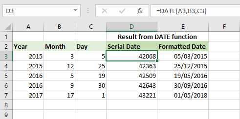
When you first put it together you may get a serial date as a return – don’t worry, just format it as a date.

Can you note something funny going on in cell B7? What’s going on there – we can’t have 17 months! Well, when there are more months than 12 (or more days than there should be for the given month), Excel adds the excess on. So in this example, it’ll take the 1st January 2017 and add 17 months onto that – which is firstly 12 months (1st January 2018) then an additional 5 months (which takes us to 1st May 2018).

Adding a number of days, months or years to the DATE Function

It’s fairly straightforward – simply add the number to the relevant argument: =DATE ( A3 +5 , B3 , C3 ) will add five years to the year in cell A3.

What if my date is in a single cell, rather than split out across three?

Good question – in this case of course it’s a serial date and our DATE function will behave a little differently.

Let’s assume our serial date is in cell A3. You would lay out your DATE like this:
= DATE ( YEAR (A3) , MONTH (A3) , DAY (A3) )
Each time we’re having to refer back to A3 for all three components of the date.

Adding, say, five years to this, it would be laid out thus:
= DATE ( YEAR (A3) +5, MONTH (A3) , DAY (A3) )

Calculating 30 days + 7 days for VAT returns

Your VAT is due one calendar month after the end of the quarter, with an additional 7 days added if you pay electronically. Let’s say our quarter ended on 30th April. Adding one calendar month gives us 31st May, and the additional 7 days gives us 7th June. This can be a bit fiddly to calculate, given that not all months have an equal number of days.

Start off by placing your quarter-end date in a cell, let’s say A1.

In the next cell, we shall use the End-of-month function, which is EOMONTH. EOMONTH has two arguments: the first is the source cell (in this case, where we typed our quarter-end date – A1). The second argument is a referer to how many months forward we want to run: 0 (zero) means the end of the current month; 1 means the end of the following month, and so on. (In fact, you can use negative numbers to count backwards by months, should you need.)

So effectively, our function will be =EOMONTH (A1, 1) because we want the end-of-month date for the following month.

Now we need to add the 7 days on. Edit your function and write +7 on the end:
=EOMONTH (A1, 1) +7

Corporation tax and Self-Assessment returns

We can use this to work out when we need to file and pay other taxes, too. The rule with Corporation Tax is payment by 9 months and submission by 12 months after the period end. Self-Assessment is a little easier as it’s just the 31st January following the end of the period to 5th April the previous year. So if you set your period end to be 5th April, you can use EOMONTH to count forward and give us the last day of the 9th month ahead.

Using this in practice

I have at work a list of clients with their period ends. In the following two columns I have formulae to calculate when tax is due for payment and when returns are due for filing. I then have a conditional format which highlights any client whose submission is due within 2 months – so I have a forward reminder of who to focus on. My conditional format uses the TODAY function, so it always updates.

Most people can remember the big annual self-assessment deadline but it might get a bit more fun when Making Tax Digital (MTD) rolls out beyond VAT. There have been suggestions that SA will become quarterly, in which case – unless HMRC sets the periods themselves (as it does at present) – it might be you really need to keep on top of when your clients’ returns are due. Having something that reminds you will become vital, so using EOMONTH may well become very familiar.

Calculating working days

Using the VAT example above, we have one calendar month + 7 days to file, plus, if paying by Direct Debit, an additional 3 working days before payment is collected. There are many other reasons why you might want to calculate working days between two dates, and there are two main ways to do it.

Networkdays

This function is very overlooked. Quite simply, you plug in a start date, an end date, and (if relevant) the number of holidays (non-working days) falling within that period, and it will tell you how many working days have elapsed.

As you can see from the image below, I have my bank holidays listed in cells F1:F8, which is the final argument of the NETWORKDAYS in cell B5. This has deducted three additional working days between 01/01/2018 and 04/04/2018.

The date in B4 is a TODAY, so the result in B5 will keep updating every time I open this spreadsheet.

Of course, my list of holidays could include staff leave as well, if I needed to work out how many days a team was spending on a project.

WORKDAY

The WORKDAY function is similar, but is based on the premise that you don’t know your end date (as you do with NETWORKDAYS), just how many days you need to work on a project (for example).

So you can see how similar this is to NETWORKDAYS – plug in a start date and a number of days on the project and you get out a date. Incidentally, in the example above, the result of my WORKDAY in cell B5 was formatted as General, so I had to go back and format it as a date.

So now you’re thinking, “OK, I’d like to have a formula that calculates that additional 3 days on the VAT submission date, how do I do that?” You’re going to think I’m thoroughly mean here as I won’t tell you… because I haven’t yet worked it out myself! I’ll ponder it, and if I nail it I shall update this post. Have a go yourself, though – remember, any kind of practice you can give yourself prior to the exam is going to stand you in excellent stead!

Calculating the difference between two dates

This is commonly used to work out how old someone is, or how long someone has been working somewhere – so it could equally apply to how old your payables are. There are two ways to do it:

1) Subtraction

As your start and end dates are both numerical, it’s possible to take one away from the other. Yes, as simple as that. However, do be warned that this might not give you the answer you expect.

Say I want to know how many days between 01-Apr and 05-Apr. If I said 05-Apr minus 01-Apr I will get the answer 4. Is that correct? Or do I need it to say 5? If so, I should say 05-Apr minus 01-Apr plus 1. The two images here should show you the difference clearly enough.

 

2) Using the DATEDIF function

This is a curious function, because it’s been left out of the Help files of most versions of Excel for at least 20 years. (From what I gather, it was originally in Lotus123 so I’m guessing it’s a ‘legacy’ function.)

History lesson aside, the syntax can be quite hard to get your head around – or at least, the final argument. Here’s the syntax:
DATEDIF ( start_date, end_date, unit )

The final argument, unit, relates to what kind of output you want – years, months or days. This is why it’s handy (I’d say essential) in calculating ages, as using other formulae or functions gives an output in days.

If we want to say how many years have elapsed, we need to say
DATEDIF ( start_date, end_date, “y” )

If we want to say how many months have elapsed, we need to say
DATEDIF ( start_date, end_date, “m” )

If we want to say how many days have elapsed, we need to say
DATEDIF ( start_date, end_date, “d” )

(Knowing how many months something is may seem a bit useless; I never came across a need for this until I started studying Level 4. I’ve discovered that how many months something happened for is necessary for certain tax calculations – particularly, what I’m thinking of is calculating PRR in a CGT calculation on the sale of a property.)

So in order to make DATEDIF more useful, we can put this together to have a formula which will return something like “18 years, 5 months and 6 days”. This will involve several steps.

To tell DATEDIF to ignore whole years and just give us the months left over:
DATEDIF ( start_date, end_date, “ym” )

On a similar basis, to ignore all the months and just give us the days left over:
DATEDIF ( start_date, end_date, “md” )

Putting a DATEDIF together

We want to say 18 years, 5 months and 6 days. The red text is our DATEDIF (we’ll need three), our green text is added so people know what they’re looking at, and we’re going to join every stage together by using a &. Here goes… it gets tricky so be careful!

A little tip: a lot of people forget to put spaces into their additional text. It’s hard to do this at first when you’re a learner, so I suggest doing everything without (in which case it’ll look like 18years,5monthsand6days) then going back and putting them in!

(Note – I know my double-quote marks are formatting badly, I apologise for that.)

To get the years: =DATEDIF ( start_date, end_date, “y” )
Then join this to the next bit: &
Then insert ” years, ”
Then join this to the next bit: &
To get the months: DATEDIF ( start_date, end_date, “ym” )
Then join this to the next bit: &
Then insert ” months, and ”
Then join this to the next bit: &
To get the days: DATEDIF ( start_date, end_date, “md” )
Then join this to the next bit: &
Then insert “days”

Put together, that looks like:
=DATEDIF(B1,B2,”y”) & ” years, “ & DATEDIF(B1,B2,”ym”) & ” months, and “ & DATEDIF(B1,B2,”md”) & ” days”

You can see what I mean that you have to be patient and careful! I usually forget a bracket or an ampersand & and have to go back and edit.

While this is a fun function to plug in your birthday and TODAY( ) and find out how many years, months and days old you are, I’m guessing you could also use it to work out a retirement date or how long someone has been on maternity or paternity leave (I don’t work in Payroll so I’m not sure about this, but I’m sure you get the idea).

Time formulae

Goodness me, I absolutely detest working with time in Excel. It’s down to the way my brain processes time, which is sturdily fixed on 60 seconds to a minute, 60 minutes to an hour, 24 hours to a day.

The way Excel processes time, on the other hand, is decimally. What I mean by this is that it takes a day and divides it by 10, 100, 1000. To understand this, go to a blank cell and type in 1.5. Now, format it as Time. Your result is 12:00:00! Have a look in the formula bar – you’ll see that it’s actually 01/01/1900 12:00:00. Well, halfway through the day is indeed midday – so of course it would end up showing 12:00:00.

So, have a think for a minute (ha ha) – what would you enter in order to have a time of 9am? 8pm? 4:35 in the afternoon? Fortunately, you don’t have to puzzle too much, because all you need to do is actually type those times in (in 24 hour clock format) and Excel will format this appropriately. Change the format back to General and you will see what it is in terms of a fraction of a day.

(If you’re curious, 4:35 pm is 0.6909722 of a day.)

If you type a time in as 0.xx then Excel will treat it as time and time alone. If you type in a time as 1.xx or 43912.xx it will take the whole number portion as a date.

Using time in spreadsheets

The biggest use of times in spreadsheets is when creating a timesheet, where staff can enter their start and end times and it will calculate how long they worked.

You need to be hyper-aware of one crucial thing if you design a timesheet: users may input time as a decimal, such that a start time of 8:30 will be input as 8.30. This will actually be read by Excel as 08/01/1900 07:12:00. Alternatively, they may read 8.5 as eight hours and fifty (or even five) minutes.

So you need to make absolutely sure you use your Data Validation settings and let users know that time must be input with a : colon.

Calculations with Time

Some older versions of Excel had an additional problem with spreadsheets tracking time. Just as with dates, to calculate how long a person worked, you take the start time away from the end time (e.g. 19:00-11:30) and that should give you how long a person worked. But what if they are shift workers? Imagine clocking on at 8pm and working through till 8am… that would give a formula of 08:00-20:00, which is impossible. In order to fix this, having the date as part of the time will help, but of course your users may find this a tremendous faff.

Secondly, when adding up all the hours over a week that a person has worked, most likely they’ll go over 24 hours if they’re a full-time worker. That means that as soon as they go over, the total cell might look like it’s deducted 24 hours altogether. For example, if you work 35 hours, then that’s 11 hours over a full 24 hours – so your total cell might give a result of 11:00 rather than 35:00.

Fortunately, time totals are now recognised as such, and will behave correctly – but you can still get formatting issues. If it does misbehave, the Custom Number Format [h]:mm should sort it.

I had a fun challenge recently, when I was commissioned to create a spreadsheet to track how many hours had been worked daily on a project and totalled for the week. This meant that instead of 9 till 5, it could be 9 till 9:30, then 10:05 to 10:25, then 12:15 to 14:00 and so on. In the end, I had to use ‘helper columns’ to assist – additional columns to do the hard work – which I then placed on another worksheet and hid so they wouldn’t be deleted by accident. (You can find about hiding and protecting worksheets here.) I’ve included this in the example spreadsheet so you can see how I went about it.

That’s it for dates and times! Remember, all you really need for the exam is TODAY() and NOW(). Hopefully you do now have a bit more understanding of the kinds of things you can do with this functionality, though.

If you’re following the suggested Learning Plan, please click here to go to the next post.

The VLOOKUP and HLOOKUP functions

Like the IF, the Lookup functions are fantastically handy. There are all sorts of ways you can harness lookups to help you speed up your work. However, like the IF, people seem to get into a terrible tangle with them to start off with – but like all functions, they have a pattern to them which makes perfect sense when you understand what it’s up to.

What does the VLOOKUP do?

Lookup functions work much like looking up a word in a dictionary to get a definition, or looking in a phone book to get a person’s number. You’re not going to get very far if you don’t know the person’s name or the word you’re trying to define – and you won’t get very far either if you haven’t got a phone book or a dictionary!

So you need two things – something to look up (person’s name), and a list of information (people’s names with their phone numbers). It doesn’t matter if what you’re looking up is a text value or a numeric value, by the way.

However, most phone books have more than one column – name, address, home phone, work phone, mobile etc – so you also need to know which column’s data you want to bring back (the column with the correct phone number in).

So that’s it – three things: the thing you’re looking up, the list you’re looking it up in, and the column your answer is in.

Syntax

We’ll look at VLOOKUP first, as it’s the commonest. It has three mandatory arguments. The final argument is supposed to be optional – remember, that’s what arguments in square brackets are – but in fact if you don’t use it you get all sorts of funny results, as I’ll show in a bit.

=VLOOKUP ( lookup_value, table_array, col_index_no, [range_lookup] )

Here we have a simple table, and at the top I want to be able to type someone’s name in and have it look up their extension number.

I start off by taking the word in B1 – Sally – over to my list in A5:B9, and then, once it’s found Sally, to return the information in the second column – her extension number. Finally, I need it to give me an exact match, as it would be irritating if it gave me the first number it felt like!

This translates into =VLOOKUP ( B1, A5:A9, 2, FALSE )

The first two arguments

lookup_value is kind of obvious. It’s the value (remember, thing you actually see in the cell – in this case the word Sally) which you want to use to look up in your table.

table_array is kind of obvious too. It’s the whole range of cells where your table sits. Bear in mind that I didn’t select A4 but started in A5. Why did I miss out the header row? Mainly because it’s not relevant – there’s nothing in there that I want to look up!

The third argument

col_index_no needs a bit of explaining. It’s short for Column Index Number. Your first column always contains what that lookup_value is going to be matched to – that’s Column Index Number 1. So if we count that as column 1, then it’s column 2 which contains our extension numbers, and 2 is what we type as our col_index_no in our function.

Remember that in our table, it’s the second column which contains our extension numbers. Don’t get hung up about it being in column B. Your table array could be anywhere!

And if we had more columns in our table, they’d each be referred to by their own col_index_no:

The fourth argument

[range_lookup] is in square brackets, so it looks like it’s optional. Without it, Excel will assume you’re looking for an approximate match – and approximate matches can be really random! You can write this argument in one of two ways:

FALSE means you’re choosing to have an exact match. You can also write it as 0 (zero).
TRUE means you’re choosing to have an approximate match. You can also write it as 1.

Here’s an example of what happens when we choose to have TRUE or an approximate match. John’s fine, as is Nigel, but Sally’s number is wrong and poor Gary and Angela don’t even get a look-in!

You’ll note that as soon as I type that last comma to go onto this final argument, I get a little panel pop up reminding me which is which, so don’t worry if you can’t remember whether it’s true or false to get an exact match. In fact, I put it into the function easily by pointing to it with my mouse and double-clicking, and it pops it straight in.

Where things go wrong

Your VLOOKUP can obviously go wrong if you ask for an approximate match in your range_lookup, rather than an exact match, as seen above. But here’s another couple of ways it can go wrong.

More than one match in column 1

We have two Johns here. The VLOOKUP will only return the first one’s number.

So remember – your first column can only contain unique values. This is why we tend to use codes, such as NI number, staff ID number, product code and so on as our first column data.

Errors in data entry

So if there are two or more identical values in column 1, we need to rethink. Just typing in John will no longer work, as that value doesn’t exist in column 1 – which is why we get the #N/A error.

So I can add in their surname initials, but then I hit another problem. Can you see why I still get a #N/A?

In this instance, John P. has a space after the full stop. I can’t see it, but it’s there. And it’s critical that it gets added in! So, data entry has to be absolutely perfect, and the presence of spaces can really throw this off.

No lookup_value

In this example, I just get going straight away with typing my VLOOKUP. However, I get a #N/A error. Why’s this? Simply because until there’s something in my lookup cell, my VLOOKUP can’t work! So all I need to do is make sure there’s something in there (in this case, cell B1) to prevent this error.

There is a way you can hide this error, so your users don’t get freaked out. You can read all about it in the next post but one.

V versus H Lookup

In the examples I’ve used, my table_array has the data in columns. This means when Excel takes the lookup_value in B1 and heads over to the table_array in A5:B9, what it’s doing is looking downwards – that is, vertically. That’s what our V stands for: vertical!

Have a guess, therefore, what H stands for…?

You’re absolutely right – it’s horizontal. An HLOOKUP is used when the data is in rows, not in columns:

This is exactly the same as what we have above, except everything’s been laid out across, rather than down. The lookup_value in A2 is still being taken over to our table_array in B4:F5, but this time Excel will start looking horizontally across row 4 to find the value ‘Nigel’.

When approximate matches are useful

It’s not always the case that we must look for exact matches. Here’s an example of where an approximate match is going to be handy. I have a list of transactions and I want to say which quarter they belong to.

I started off by having the start and end dates of each quarter in a little table, plus of course which quarter the dates refer to.

Then below, I could set up a VLOOKUP to pull out the quarter each transaction belongs to.

(As you can see, I also needed to use another tool that we looked at a while back – absolutes. Do pop back and have a quick read through if you’re at a loss as to what I mean.)

So as you can see, sometimes approximate matches are really handy! Just make sure your table_array is sorted in ascending order otherwise it might go a bit funny.

Combining other features of Excel

• You can make your life a lot easier by naming the lookup_value and the table_array and using those names in your function.
• If you suspect your table_array will grow, for instance if you import extra data or need to add more lines, then format your table_array as a data table.
• You can use Data Validation to create a drop-down list of expected values for your lookup_value. Where would you find the source cells for this? Why, in the first column of your table_array! Furthermore, if you’ve formatted the table_array as a data table, any extra rows you add to the end automatically add themselves to the drop-down list.
• You can have your table_array on another worksheet and link across. The only problem with this is you can’t always see if you’re getting the right col_index_no, so it’s useful to make a note first. (If you’re following the suggested learning plan, we haven’t got that far yet – bear with!)
• You can use password protection to prevent someone accidentally deleting your carefully crafted VLOOKUP.

Considering that by now you know how to do all but one of the above, you can immediately make any spreadsheet containing a VLOOKUP seriously powerful.

‘Reverse’ lookups

It would have made more sense to have the above example, with the Quarter 1, Quarter 2 etc, arranged in a slightly different way. Rather than having start date | end date | name of quarter, it would look more logical to be arranged like this:

However, VLOOKUP is programmed to look down the first column of a table_array. As the first column contains text, this is no use if we’re trying to look up dates. In this instance, we’d need to look up in col_index_no 2 and ‘reverse’ to col_index_no 1.

The short answer is yes – it can be done. You can look up to the left of your Lookup column, not just to the right.

The long answer is that firstly it’s way beyond the scope of what AAT will be asking you to do; and secondly it either involves the use of two other functions or an array formula (which is a special kind of formula with magic in it). I won’t be covering it here, but I do believe it’s useful to at least know that things can be done in case you ever need.

Further reading

Here is a very interesting article on how not to mess up with VLOOKUP. It explains the basic syntax then outlines a few problems, such as what happens if you insert or delete a column from your table_array. Well worth a read if you want to extend your knowledge!

Your turn

I have a nice set of exercises for you to practise everything, also involving some of the other features I mentioned above. Have fun – VLOOKUPs are awesome! You can download them all from here.

If you’re following the suggested Learning Plan, please click here to go to the next post.

Nesting IFs

I always think that ‘nesting’ functions sounds kind of like birds getting all comfy for the winter, but disappointingly it’s much more prosaic than that. ‘Nesting’ is essentially putting one function in its entirety into another function – which we saw in action in the last post. (In fact, if you haven’t read it yet, it might help if you do.)

Big important note which you must read!

I mentioned all the way back here that it was pretty important to type your formulae out, rather than using the function builders which you get when you select a function from the Formulas tab. What you’re about to learn here cannot be done via those function builders. You just can’t. THIS is why I was so adamant that you should stop using them, if you’re in the habit, and learn to write them out. I even checked on my advanced Excel users group and they agree, there’s no way you can do it unless you type it out. Sorry!

Why nest the IF?

You may remember me saying that an IF statement is an either/or situation. We have a logical test, or statement, then we have what to do if that logical test is true and what to do if it’s false. That’s great if you only have two things.

But what if you have more than two? Life is rarely simple enough that we just have a this-or-that situation going on. We need to have shades of grey between the black and the white – and that’s when a Nested If would step into the breach: you put an IF inside another IF.

The example I’m going to use here is the grading system AAT introduced with AQ2016. Before, you either passed or failed – which was perfect for an IF; but now you can have pass, merit, distinction or fail – which is perfect for a Nested If.

Get organised

The first thing you have to do with a Nested If is to organise your shades of grey. You have to think carefully in top-to-bottom or bottom-to-top order. Thinking of our results, anything 90 or above is a distinction, 80 to 89 a merit, 70 to 79 a pass and below 70 is a fail. We’re going to set it up so that our score tries itself for size in the first level. If it doesn’t fit, it’ll try the next level; and so on, until it finds the perfect match.

On that basis, if we had our different levels all jumbled up, our score would have a devil’s own job trying to find which one it fits into, so it’s essential we get organised.

I was taught top-to-bottom (larger numbers to smaller numbers), so that’s the way I’ll show you here. Others are taught the other way up. Remember I said in the IF lesson that whatever you write it’s essential to look at your answer and see if it’s what you’re expecting – if you’re testing something is bigger than 5 and it turns out to be working on numbers smaller than 5 you know you’ve messed up somewhere! Same thing here. Test your function by trying various inputs and see if the output is correct. So if you go bottom-up rather than top-down, it doesn’t matter – just test it to check!

Laying out your function

Let’s think about the syntax for a minute. We’d normally have 3 arguments:
=IF ( logical_test, value_if_true, value_if_false )

Using our AAT exam results example, that would mean something like: IF the score in cell A1 is greater than or equal to 90, say “Distinction”, otherwise say “Merit”. But that suggests that everything below 90 is a Merit, which isn’t the case. So the problem here lies with our final argument, our value_if_false, because we could have more than one. It’s at this point we’ll nest an If.

So what we actually need to say is, IF the score in A1 is greater than or equal to 90, say “Distinction”. IF NOT, then IF the score in A1 is greater than or equal to 80, say “Merit”, otherwise say “Pass”. But again, that suggests that everything below 80 is a pass, so we’d need yet another Nested If!

So our final version is: IF the score in A1 is greater than or equal to 90, say “Distinction”. IF NOT, then IF the score in A1 is greater than or equal to 80, say “Merit”. IF NOT, then IF the score in A1 is greater than equal to 70, say “Pass”, otherwise say “Fail”.

You can visualise the decision-making process like this:

‘Translating’ into Excel-speak

Looking at the above, we need now to write it out in actual Excel-speak, so we can use it for real. Personally, I find it easier to break down a Nested If by writing each different level as a separate line – visually, it just makes more sense. You may find your own trick to keeping each level distinct – whatever works for you. 🙂

=IF ( A1 >= 90, “Distinction”,

IF ( A1 >= 80, “Merit”,

IF ( A1 >= 70, “Pass”,

“Fail” ) ) )

Written out in the Formula Bar it’ll look like this:

=IF(A1>=90,"Distinction",IF(A1>=80,"Merit",IF(A1>=70,"Pass","Fail")))

It looks a bit crazy, but as you type it, your guiding panel will help you. Just remember to move straight onto the next IF rather than the value_if_false, until your very last level. (Note: If the animated gif doesn’t show so well, download a PowerPoint file of it here.)

Important notes

• You only need one = at the start. Don’t keep putting more in, you’ll upset Excel.

• Each bracket you open needs a close bracket – which all go right at the very end. Watch carefully as you pair them up, as they’ll briefly go bold as they pair. I look to the very first open bracket and when I see that’s gone bold I know I’ve done enough. They also colour-code as well which is handy.

• For however many levels you have, subtract 1. That is the number of IFs you’ll need. For instance, here we have 4 levels therefore that’s 3 IFs. What I see lots of people do is get to the final level, and (continuing from above), say if A1 is less than 70, say “Fail”, but then … otherwise, what? You only need one final value_if_false, right at the very end.

When it all goes wrong

• The main reasons nested IFs fail is because of a missing comma. You have to be so careful to separate out each of your arguments with commas and they’re not that big on the screen so it can be so hard to see what you’ve done. When you confirm, you’ll get an error message, but Excel will often shade over the part it detects a problem with. In this example here I removed the second comma, thus ‘blurring’ the first value_if_true with the start of the second IF. But Excel has indicated the exact area of the issue.

• Another common error is missing brackets. Excel calls these parentheses, so if you get the following error, check your brackets are a) in the right place and b) paired, one opening for one closing in every case.

• It’s a classic mistake, with all your worry about brackets and commas, to completely forget to put your text in double quotes. If that happens, you’ll get the #NAME? error.
• Still getting stuck? Move right to the very start of your entire formula and type ‘ (a single quotation mark). This turns everything in the cell into text, and has the advantage that you can finally park it and walk away. There have been many times where I’ve been flummoxed by a problem and each time I’ve confirmed it’s thrown up another error, thus trapping me into a cycle of fix-error-fix-error. Before you get to the point of throwing your computer out of the window, STOP! Pop a single quote in, save your spreadsheet, take a deep breath and do something completely different. Your brain will thank you for it!

An alternative to a nested IF

You can nest up to 64 IFs – although the idea of doing this hurts my head! Oh my goodness, the brackets at the end! You have to admit, doing more than about 5 or 6 is a bit bonkers. So what could you do if you have more than a reasonable amount of options you need to return? Quite simply, use a VLOOKUP. A lot of people will just go straight for the lookup and not even bother with a nested IF.

However, nested IFs are useful for two reasons: firstly with a VLOOKUP you have to have a table somewhere with your lookup values in. Supposing a user finds it, and deletes it? If you have everything ‘hard-coded’ in a nested IF, that’s less likely to happen – and if you just have the single function rather than a separate table elsewhere, it’s easier to protect and lock down.

Secondly, and more critically, you can’t test for multiple conditions in a VLOOKUP. Supposing you need to check if you got more than 70 in two subjects in order to pass? (If you need to do this, see this post.) A VLOOKUP can’t look up more than a single value.

But I think ultimately it comes down to preference. Some people I know use lookups everywhere; me I’m more of an IF person!

Over to you

Download some exercises here (three worksheets in the one workbook). Bear in mind there are several different ways you can complete the exercises – I’ve given some variations on the theme in the answers but you might have come up with another version again – this is absolutely fine, you get Smug Points for a formula that works, not a formula that’s a carbon copy of mine!

The following post expands on the principle of nesting and gives some great additional directions in which you can take your spreadsheets. I’d very much recommend them to anyone who is already pretty clued up on Excel. However, what’s covered is not part of the AAT synoptic, so if you are pressed for time you can skip it.

To learn more about nesting, click here.
To continue with the suggested learning plan, click here.