Getting to grips with Functions

Functions are absolutely the bedrock of Getting Things Done in Excel. They are so, so useful! Here, we’ll have a look at a few of the commonest functions – ones which you probably already know – just to lay the ground for a deeper understanding in following posts.

Firstly, what is the difference between a formula and a function? Well, functions all start with = so in fact they’re all formulae. Functions are a large collection of built-in formulae in Excel, all pre-programmed to do something specific. You can use them on their own or in conjunction, or even inside each other, to make a huge range of tools available. You can’t use a function designed for one thing, to do something else. Chances are, if you need your function to work in a different way, you need a different function.

Let’s have a look at SUM and branch out from there.

In the above gif, I make reference to typing all my functions. Sure, it’s what the pro users do, but that’s not the only reason. There are certain instances where you can’t insert a function without typing. These are covered briefly in the next post.

Further functions

In the next gif, you can learn a bit more about some other basic but extremely useful functions.

Even more you can do with functions

So far, we’ve looked at having a range of cells as the input in our functions, such as A1:A3. In the next gif, you will learn how you don’t have to stick with just a range, but can have a whole mix. Here are some examples to look at before you watch the gif.

Numbers alone	=AVERAGE (33, 44, 55)
Cell references alone	=AVERAGE (A1, A2, A3)
Ranges alone	=AVERAGE (A1:A3) =AVERAGE (A1:A3, B10:B15)
Numbers with ranges, ranges with cell references, cell references with numbers	=AVERAGE (55, A1:A3) =AVERAGE (A1:A3, B10) =AVERAGE (B10, 55)
Numbers AND ranges AND cell references	=AVERAGE (55, A1:A3, B10)

Have a go!

I have a few files in which you can have a go at practising your basic formulae and functions (and yes, I include the answers!).

This link is for a folder on my Google Drive which consists of a pdf with the Exercises in, three spreadsheets you’ll need to use, and three answer spreadsheets (no peeking!). It’ll download as a zip file, so once it’s downloaded, right-click on it and choose Unzip to be able to access them all.

Good luck – and remember, please contact me if you’re feeling at all befuddled!

If you’re following the suggested Learning Plan, please click here to go to the next post.

More about Functions

Having looked at a few basic functions in the last post, and learnt a little bit more about how we can extend them from the basic single range input, we’ll now start to have a look under the bonnet of this valuable set of Excel tools.

The layout of functions – syntax

As I explained in the previous post, a function is pre-programmed to do a very specific task. Estimates vary, but there’s more than 400 of them – and if there’s something you need to do that doesn’t seem to have a function already, you can usually find an add-on or even write your own! They come in categories, such as Statistical, Engineering or Financial, which can help you if you’re browsing to find something that does what you want – but you absolutely don’t have to learn them all to be ‘good at’ Excel.

Now – functions all have a very specific layout to them. Once you grasp that, you can get the gist of loads of them. Let me explain.

Take normal old SUM. It’s =SUM(A1:A10)
Average is similar: =AVERAGE(A1:A10)
So is Max: =MAX(A1:A10)
And Min, and Count, and CountA…

They all have this same pattern:

1. equals sign – they’re all formulae
2. a name. You have to get this right, otherwise Excel won’t understand what you’re after
3. an open-bracket
4. bits between the brackets – these are called arguments and give Excel more detail about what you want to do with the function. You can have one argument, two arguments, sometimes even up to 255! They are always separated by commas. Some functions actually work without any arguments at all!
5. and a close-bracket.

The entire caboodle is known as syntax. You have to get the whole syntax correct for Excel to play nicely. If you don’t, however, you can often get clues as to what to do to fix it.

Now: the bits between the brackets – arguments. Most people think that SUM only has one argument, a range (e.g. A1:A10 – a group of cells, in other words). In fact, you can have loads, as we saw in the previous post. You could say (A1,A6) or (4,8,10) or even a mix (A1,5,B2:G15). Whatever you have, all SUM can ever do is add. That’s what it’s for.

It may sound silly to say this, because everyone knows SUM, right? But I still see =SUM(D1-B1). Why not just have =D1-B1? Or in other words, why are you telling an adding function to subtract?

So understanding that each function is designed for one thing and one thing only is actually really important.

Now to dig into this a little bit more, what I’d like you to do is to open Excel and press F1. This opens your Help files. Type in SUM function and it should appear. Below a brief bit of information about what it does, look for where it says syntax. See if you can understand the explanation. You can see it refers to arguments – remember, the bits between the brackets: the first argument is required, but the next – and subsequent 253 – are optional. So – 255 different numbers/ranges/cell references in total – wow! Suddenly our humble SUM is looking quite sophisticated!

More key terminology

At this point it’s really important to understand another key word: value. It’s a funny word that pops up often. What it is is actually any one of several things:

• text
• number (called ‘numeric’)
• text and numbers together (called ‘alphanumeric’)
• the answer to a formula or function.

I’d like you to focus on the last one for a moment: the answer to a formula or function. Think about a cell with a formula or function in it. Where do you see the actual formula? In the long white bar above your cells – the Formula Bar. And where’s the answer? Well duh, you’re thinking, it’s in the cell! But then, surely the formula is in the cell? But NO: here’s a critical distinction: you SEE the formula elsewhere – what you actually SEE in the CELL is the value.

A value is “what you see in the cell”. This is going to be particularly relevant when we look at IF statements and VLOOKUPs.

How Excel helps you when you’re writing a function

Now, think about when you start typing a function. As soon as you finish typing the name (SUM, COUNTIF, VLOOKUP, etc) and type that open bracket, you get a little panel appear under what you’re typing.

This is a guide to the syntax, and tells you what arguments you need. The argument which is bold is the one you’re currently writing. Anything in [ ] is an optional argument.

A big tip

I appreciate that so far I’ve been telling you to type or write your functions, and I’m fully aware there’s a nifty little tool which will help you build your function from any of the Function drop-downs on the Formulas ribbon. I really don’t advocate using this. (If you’re wondering what I’m talking about here, I’m actually not going to tell you because it will lead you up the garden path.)

Firstly, I’ve learnt from experience that students/delegates rarely get a proper sense of what they’re doing if they’re just filling in boxes. By actually typing and thinking hard about what you do, you learn much more effectively.

Secondly, with more complex functions (such as nesting, which you can read about here), you just can’t do this any other way – you have to type.

Learning a little bit more

Now, what I’d like you to do is slowly and patiently go through the Help files searching for each of the following in turn. Type NAME function in each case (for instance, SUM function or MAX function) to find them. Read the description. Look at the syntax. What clues are there in the arguments, words like ‘range’ and ‘value’, that can give you pointers?

Try these for size:

• PROPER
• CONCATENATE
• SQRT
• PRODUCT
• INT
• ROMAN

You’ll probably find you can understand every single one!

Go on, give it a try! Report back and let me know 🙂

If you’re following the suggested Learning Plan, please click here to go to the next post.

Useful Files

You may find the following files useful. They’re all in pdf format.

1. Dictionary of Excel terminology and explanations of Error Codes – don’t know your range from your value? Worried about your #div/0? Check this out.
2. Keyboard shortcuts you can use in Excel. I use a lot of these – particularly the shortcut for entering today’s date, for zipping up and down through the different worksheets, for editing a cell’s contents and for applying absolutes.
3. Exam specification. Link to follow – I’m in the process of updating these pages.
4. The suggested Learning Plan, if you haven’t already found it. Use it to keep track of your development, or as a reference to make sure you cover everything you need.

If you’re following the suggested Learning Plan, please click here to go to the next post.

Data integrity

Before you do anything fun like charts, sorting, pivot tables or what-have-you, I’d like you to turn your attention to the gritty subject of data integrity.

What is data integrity? Basically, there are certain ways Excel expects data to be presented in order to harness certain tools, and if you get it right, you can save a barrel of time. Essentially, it boils down to two things:

1. Elimination or minimisation of errors
2. Quicker use of tools and features

I’ve tried to think of others, but they all come down to this in some way or another. And let’s face it – both of these are going to be pretty high on your agenda in the exam, right?

An example of bad data integrity

It’ll help you enormously if you can see it done incorrectly first. This is a real-life, genuine spreadsheet put together by someone doing their best but in desperate need of Excel training! Download the spreadsheet here.

I’d like you to pause for a couple of minutes and make a few notes about what’s wrong with it.

Had a chance to think about it? You probably noticed things like:

• Random colour-coding – why?
• Dates are not put in correctly (you should always put / instead of . in dates)
• Gaps in the data – blank rows and columns
• Column headings are missing – if we didn’t have the title VAT would we know we were looking at money in columns F, G and H?
• Errors – did you notice the year .45 in cell M18? And the spelling mistake in N8? And is DEPt supposed to be Dept, or DEPT?
• Is there any reason behind the split? Why not have all the data together?
• Random border formatting

The problem with all of these is if you want to get any meaning out of it, or even to do any data verification, it’s really hard. Now we’ll look at how to fix these kinds of things.

An example of competent data integrity

Now download this spreadsheet, which is the same data as the previous one but the following year. You’ll notice an immediate difference:

• The data is all in one block (range) of cells.
• There’s a key at the top to tell you what you’re looking at.
• Data has been correctly formatted – dates, currency, etc.
• Filters have been applied, so you can quickly sort or burrow into your data to extract meaning.
• The range has been formatted as a Table (this isn’t essential, but can help).
• There’s a unique code to each line (this isn’t essential, but certainly helps!).

Why does this all matter?

For a start, the latter is a whole lot more workable. A spreadsheet is pointless if you can’t get any information out of it. Imagine a dictionary where all the words are in random order!

Secondly, data in a whole range with no blank rows or columns means you can use Autofill, Sort, Filter, Pivot tables, Charts, Subtotals… AND you can apply these tools in lightning quick time!

Try it: click anywhere in the range of cells. Anywhere, just a single cell. Now go to the Home tab, if you’re not already on it, and click Sort & Filter, Custom Sort. See how the entire range of cells has been automatically highlighted for you? Hey, neat! No more endless clicking-and-dragging down hundreds of rows!

So: the lessons to learn here…

1. Always have column headings
2. Never have completely blank rows or columns (Please also see note below.)
3. Format your data appropriately
4. Check for errors
5. Include a key or notes to explain aspects if needed.

And additionally, but not essential,

1. Widen all columns to fit all the data, if it’s not going to leave the columns stupidly wide (and use Wrap Text if it’s appropriate)
2. Have some kind of unique reference for each line, if appropriate, to aid data checking or looking things up
3. Use features like Freeze Panes if it helps
4. Put the formula(e) at the top, to allow your spreadsheet to grow (and so that it’s on display all the time, instead of having to scroll for it). See Spreadsheet design for more info on this.

I hope these considerations help when it comes to designing a really useful spreadsheet!

Please note

Over the years I’ve been training, I’ve seen all manner of learning materials, and a great many sample spreadsheets for you to work on have completely blank rows or columns. This does, it has to be said, make my teeth itch. The functionality of tools such as Sort, Charting, Pivot Tables can be hindered by the presence of blank rows and columns. It’s not that they won’t work, but that the functionality becomes cumbersome. The problem with this is it forces the user to select (highlight) all the data – this is fine if you only have a little spreadsheet, but I’ve dealt with some whopping huge spreadsheets over the years. In other words, by having blank rows and columns in learning materials, you are being taught to make your life harder.

Excel was designed with a seriously neat feature – rather than selecting all the data, all you need to do is have your active cell (the one with the thick black border around it) somewhere in your data, and when you use any of the Data tools Excel will work out how big your data is, automatically. How cool is that? So why, why on earth would you make your life harder by having blank rows or columns?

Visually, if you want to have the appearance of blank rows or columns, you can – just use your formatting/column width/row height tools.

Anyway – my pedantry and frustration aside – please note that if you set about deleting these naughty blanks in your example spreadsheets, your answer may look substantially different from the example answer, which I can imagine would be pretty confusing – so it would be really unfair of me to insist you have to do this in all cases. I guess, if it’s the real world, delete delete! But if it’s learning materials, grin and bear it. 😀

Adopting a spreadsheet from someone else

I’ve put together a little guide on what to do if you have to start working with a spreadsheet that someone else designed, which is cumbersome or irritating to use. Have a peep here if you’re so inclined – but it has nothing to do with the exam, so don’t worry about it if you’re here for studying only.

If you’re following the suggested Learning Plan, please click here to go to the next post.

Spreadsheet design

In your exam, you’ll be asked to put together a small spreadsheet consisting of one of the elements you learn in the other units – it could be something like partnership profit distribution or a small budget or cash flow. It’s worth, therefore, considering a few of the design principles behind a decent spreadsheet.

At this juncture, I want to stress one very important thing: NEVER have data in a formula. For instance, if you have a formula multiplying a cell value by the VAT rate, =B6*20%, what happens if the VAT rate changes? Far better to have the VAT rate in a separate cell, so your formula says (e.g.) =B6*G1. That way, all you need to do is amend cell G1 with the new VAT rate and everything should cascade down. Learn how to do this here.

1. Top of the list is what do you want your spreadsheet to do? Is it a place to get calculations done, or to store data for further processing elsewhere? What kind of data will go into the spreadsheet, what information do you want to get out of it? Once you know this, you can then think about…
2. The layout. Commonly we have titles at the top and sides, data in the middle and formulae at the bottom and/or right. Sometimes I sketch out on paper what I need to achieve, before I start typing away and have to rehash it several times before I’m happy with what I get.
3. Next, think about what type of data is being presented. Will that mean you have to lay it out in a different way from how you first imagined? Sometimes your spreadsheet works better, for instance, with months across the top; sometimes, with months down the side.
4. Use as little formatting as possible. It adds unnecessary bulk to your file size, it can make it harder to read (I personally hate it when people overlay the perfectly useful grid with a black grid, it does my eyes in) and you can seriously waste time – especially, don’t get distracted with the pretty-pretty when you don’t have the time to waste in the exam.
5. Now, it’s worth thinking about the user. Will your users be good with Excel, will they be freaked out by your advanced formulae, would it actually work better to have a series of formulae which calculate in steps, so people can see how you’re thinking? Will you be able to remember what your formula does in six months?!
6. Should you restrict data entry, so accuracy is maintained? Think about no. 5 at this point – sometimes, restrictions have led users to tell me the spreadsheet is ‘broken’. I have been known to have a little note somewhere saying ‘Don’t panic, you will only be able to click into certain cells – this is to prevent accidental overwriting, it doesn’t mean it’s broken!’ just to reassure the beginner users! However, you can use in-cell drop down choices, password protection, cell locking and so on to guide people.
7. Design your spreadsheet with long-term use in mind. As an advanced user, I find it frustrating when the spreadsheets for y/e 2014, y/e 2015 and y/e 2016 are all slightly different just because the design’s not flexible enough – it means year-on-year comparison is harder than it should be. If your data accumulates by the month, you can actually have your formulae at the top. In this image, that’s what I’ve done: the formulae will have cell references like A4 to A100000 so there’s no possible way my data will get missed out. (Unless I really will have more than 100,000 rows, in which case… but I’m sure you get the idea!) I have also used Freeze Panes to allow for useful scrolling – see here for an explanation of what that is and how you do it.
8. Can you write any explanatory notes to help explain what you’re doing, such as colour-coding? I quite often have a final column at the end of all my data called Notes where I describe what the data is, where I got the data from, maybe who to contact for queries… anything to help out. I must admit I’m more pragmatic than considerate at this point: I’ve wasted way too many hours over the years fixing the problems users have created, so I try and make it as easy an experience for them as I can to save myself hassle further down the line!

Being consistent, being methodical and keeping it simple are often the ways to go with the best spreadsheets. Seek guidance from those you work with and learn from the messes other people make (heh!). I’ll leave you with two things: Firstly the ICAEW’s excellent Twenty Principles for Good Spreadsheet Practice (pdf), and secondly, the cautionary observation that as slick and trick as I am with my Excel, I have often got myself in a stupid tangle just simply because I’m being too clever. Don’t be a smart alec like me!

I’ve put together a little guide on what to do if you have to start working with a spreadsheet that someone else designed, which is cumbersome or irritating to use. Have a peep here if you’re so inclined – but it has nothing to do with the exam, so don’t worry about it if you’re here for studying only.

If you’re following the suggested Learning Plan, please click here to go to the next post.

Useful tools and features

Here are a few little tips for making your life quicker and easier when using Excel. It’s great when you know about them, as it can make you look like a real Excel pro!

Autofill 1

When you enter data into a cell, look carefully at the border. In the bottom right-hand corner of the active cell, you can see a small blob. When you pass your mouse over it, it becomes a baby plus – this is different from the big plus you normally get when you move your mouse over the spreadsheet.

This baby plus is called Autofill and lets you access all kinds of useful things!

First up in the demonstration gif (see below) is months and days. You can see at the bottom of where you stop dragging, you get a small square. I call it the Box of Tricks (but officially it’s called Autofill Options). You can see you can either have the original cell copied all the way down, or have alternatives like filling only with weekdays. So handy!

It works with numbers too. Stepping into your Box of Tricks allows you to choose to fill a series or to copy the cells, just as before. If you need to put in a different series, you have to give it the first two numbers, select them both, then drag with your Autofill.

You can see this works with dates as well. Incidentally, I used a keyboard shortcut to put in today’s date automatically: hold the Ctrl key down and press the ; key once and you will get today’s date! Ta-da!

Autofill 2

But wait! There’s more!

If you want to copy without including the formatting, you can do that too! This can be really handy if you don’t want to mess up a formula or overwrite text.

And here’s a real timesaver – if you have ANY data to your left, double-clicking your baby plus will snap your series straight down the same number of rows. Try it… How cool is that! If you’re like me, working on spreadsheets with thousands of rows, this can be a genius tool and no mistake.

Also, you can harness it in your formulae – probably the commonest use for Autofill. When you double-click or drag a formula down, any cells referred to in the formula will change as you go down.

And you can also use it to copy formatting over text, using your Box of Tricks. Huzzah!

Autofill 3

With Autofill, you don’t just have to drag down – you can drag across.

However, with a large number such as a date, you might get a bit of a hoohah going on in your cells, as can be seen here! But wait – when I look in the formula bar everything’s there, so what’s going on? Don’t panic, all it means is that the cell isn’t wide enough to show the whole number. Rather than showing you a portion and fooling you into thinking that’s the whole number, it puts a row of ### to warn you. Just widen the column!

As you can see here, you can widen the columns neatly by double-clicking on the boundary between one column letter and the next. If you have several to do at once, select all of them and double-click any of the boundaries.

I also did a formula here to add 7 days onto each of my dates. I just dragged the formula across instead of down, and hey presto! I have a week later on each of my dates!

‘Gluing’ a whole row in place (Freeze Panes)

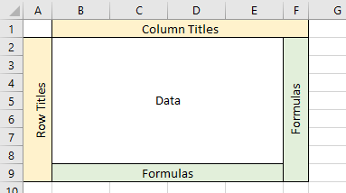
This feature is surprisingly underused. Basically when you set up a spreadsheet, you’ll have column headings at the top, to tell you what’s in your columns. But when you scroll down, they can disappear off the top of the screen – which isn’t so useful!

To fix this, you can ‘glue’ rows in place so that no matter how far down you scroll, you can still see your column headings. This is called Freeze Panes.

You can also do this with row headings, so if you scroll off to the right they’re still in place.

The gif of this is very wide and won’t display properly here, so I have uploaded it to my Google Drive. You can see it here. Remember, please download it – it won’t play in Google Drive as is.

The opposite – removing the Freeze Panes – (disappointingly) isn’t called Thaw, but Unfreeze. Grammarians, look away now!

Hiding columns or rows

There may come a time when your spreadsheet is a bit unwieldy and you have too many columns or rows to be able to see clearly or navigate effectively. You might also need to show someone something but not wish to display data which might be confidential. When this happens, it may help to hide some rows or columns. This is like folding the columns and rows out of the way, it is not the same as deleting.

All the instructions here refer to columns, but they equally apply to rows.

• To hide: Firstly, select the entire column(s) you want to hide. Right click somewhere in the highlighted bit, and choose Hide. Note that there’s a pair of little lines as the boundary between the columns now, whereas before it was a single line. This is a clue that columns have been hidden.
• To unhide (reveal them again): Select BOTH columns (or rows) either side of the hidden column, right click somewhere in the highlighted bit, and choose Unhide.
• To unhide many columns at once: Select over all the columns concerned. Right click as before, and choose Unhide.
• To unhide Column A (or row 1): If your very first column(s) or row(s) have been hidden, you have to click and hold, and move back to the left. Then you can right click and Unhide. For Row 1, obviously you click and drag upwards.
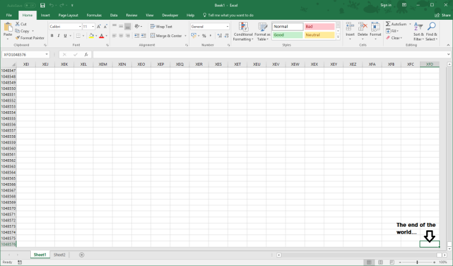
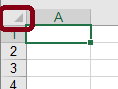
• To unhide everything that’s hidden, in one go: Click to the left of the column letters and ‘north’ of your rows, on the small square with a triangle in – this selects your entire spreadsheet and is very handy to know about – then you can double-click as if to widen the columns, and everything gets Unhidden. Remember to do the same for the rows.

Flash Fill

This is a stupendously fab tool, which very few people seem to know about. It works by recognising a pattern and projecting the pattern all the way down all the rows.

In this example, I want to have a column with full names, rather than just one for First name and one for Surname. (Incidentally, Surname is a British term meaning family name or last name.) I start off by typing the first in the pattern, with a space as needed. Then I start typing for the next row – and before I’ve even got two characters in, it’s recognising what I want to do!

All I need to do now is press Enter to confirm it, and bingo! It’s done! Cool, hey?

 

If you’re following the suggested Learning Plan, please click here to go to the next post.

Getting to grips with Formatting

Formatting is one of those tools which catches many people out, because there are some rules of data entry which aren’t always made clear to beginners.

Part 1 – the basics

Firstly, as you can see in this gif, text always aligns to the left. If you have a mix of text and numbers – called alphanumeric – then it’ll align to the left.

Secondly, all numeric data aligns to the right. This includes dates and times, because behind the scenes, they are stored as numbers.

So why should I care? If you have a long column of numbers and you suddenly spot something is over on the left, you’ve done something which makes Excel think it’s text. It’s a handy little feature for checking your data entry! Common mistakes might be having two dots in a number 52.31. instead of 52.31 or putting an O or o instead of a 0 (they’re actually pretty close on the keyboard, so this is commoner than you’d think).

So the big thing about this is, to start with at least, don’t overrule the default alignment – it can really help with spotting initial errors.

Part 2 – number formatting

In the following gif, I’ve walked through all of the commonest types of number formatting.

1. In cell A1, I show you simple General number formatting, which then allows you to be able to increase or decrease your decimal places quickly.
2. In cell A2, I apply Currency style formatting. As you can see, you automatically get a £ sign. (If you’re in a different country, your default currency symbol might be a $ or a €.)
3. In cell A3, I apply a related format – Accounting. As you can see, the big difference is where your currency symbol is. With Acounting, it’s always way over on the left of the cell.
4. In cell A4, I again apply Currency formatting. Now you can see an additional feature of the Accounting format – it’s set in a little bit from the right hand side. This is so that positive and negative numbers will still line up if you choose to show negatives in brackets rather than with a minus sign (1.00) rather than -1.00. I’ve covered how to do brackets in another post.
5. In cell C1, I show you a formula which has been set up to calculate a percentage. It divides A2 by A4 then multiplies by 100, which is what we do for a percentage, right? However, it looks like a normal number which could cause other users to think it’s something else, like money with a crazy amount of decimal places rather than an actual percentage. So…
6. …in cell C2, rather than multiply by 100, I apply the Percentage formatting style. Now you can see I have a % symbol, and of course I can adjust the decimal places up and down. Note that as I adjust the decimal places, Excel automatically rounds up or down as appropriate.
7. In cell C4, I apply Comma Style formatting, which places what’s called a ‘thousands separator’ in the number. Basically instead of 1234567 it shows 1,234,567 i.e. it’s separating the thousands with a comma. Applying this format automatically gives you two decimal places too, by the way.
8. In cell E1 I show how not to enter a date. It seems surprisingly common to do dates this way, but as you can see, Excel treats it as text. The problem with this is if you want it to display in different ways, or even if you want to perform a calculation off the back of it. You could have a formula referring to the date saying +30 which would give you the latest date you’d need to apply for VAT if your turnover has gone over the threshold, for example. Very useful!
9. In cell E2 I show you how it should be done. You use / (forward slash, never backslash) and it will automatically recognise that as a date. You can then apply a different form of formatting on it – here I choose Long Date which gives me the whole month name and the day with a leading zero (01 instead of just 1).
10. In cell E7 I show you how not to enter time. Don’t use dots, because Excel treats it as a basic old number! Again, if you want to do calculations based off this, such as in timesheets, you’ve painted yourself into a very irritating corner. (Can you tell I’ve done this before?!)
11. In cell E8 I show you how it should be done. Use the colon : to separate out your hours from your minutes. You can even apply formatting which will show the seconds, too.

Part 3 – getting rid

It’s important to bear in mind that your cell formatting is separate from the cell contents.

It’s sometimes been the case that I’ve been working away on a spreadsheet and suddenly one of my cells has formatted to a percentage or it’s gone blue or something. This is likely to be because someone was ‘doodling’ in a little corner of the spreadsheet, applied formatting, then later cleared the cell’s contents.

However, unbeknownst to you the formatting has been left behind, invisible, waiting to surprise you when you next put something in that cell!

If you want to strip off all formatting quickly and easily, go to your Home tab if you’re not already there, then have a look way off on the right of the ribbon – you’ll see a small button with a pink eraser called Clear. Click it for various options. I use this quite a bit.

Do have a play with a blank spreadsheet and all the different number format options.

Note in particular that when you apply Percentage formatting, it removes the need for you to have to multiply by 100 – that’s part and parcel of the formatting. I do sometimes forget even now, and then I end up with a ludicrously large percentage! Just remove the *100 from your formula.

Note also that when applying Time formatting, you need to train other users of the spreadsheet to recognise the importance of entering time how Excel requires, and not how they might be inclined to enter it.  As an example imagine someone put 12.5 to mean ‘half past twelve’. Imagine then that someone has formatted it to have 2 decimal places (12.50). Can you see how that could easily be interpreted as “fifty minutes past twelve”, and not “half past twelve”? If you’re setting up timesheets it’s essential that you train people first. It’s in their interests anyway – a timesheet which Excel thinks is actually twelve fifty rather than twelve thirty might have cheated them of 20 minutes of pay (or worse, suggested that they worked 20 minutes longer than they actually did).

If you’re following the suggested Learning Plan, please click here to go to the next post.

Getting to grips with Formulae

Formulae? Formulas? I say the former because I’m British, but Excel is an American program so hey, I say the latter too. Whatevs! If you’re new to formulae in Excel, let’s get you going!

Think about doing something like 2 + 3 on a calculator. What buttons do you press? Literally, 2 then a + then a 3, then the =, right?

In Excel it’s exactly the same, but with one crucial difference. In Excel, all formulae start with the =. As soon as you type that, Excel recognises you’re typing a formula.

HYPER IMPORTANT DO-NOT-IGNORE INSTRUCTION TO FOLLOW!!

Excel is VERY specific about one key instruction you give it when you’ve typed your formula. You MUST confirm to Excel that you’re done typing and want it to give you the answer.

When you start typing in a cell, your Status Bar (the bit at the bottom) helpfully says Enter, because it wants to remind you that when you’re done typing, you need to press the Enter key. Alternatively, if you’re a mouse user, you can click the Tick on the formula bar. When you point to the tick and wait, it helpfully tells you Enter – again, reminding you of what to do.

This little animated gif shows you how. It also shows you what to do if you start typing and change your mind – just click the x.

So – to confirm, Press Enter OR Click The Tick. I don’t care which you do, just, for the love of all things mathematical NEVER ‘CLICK OUT’, i.e. NEVER click anywhere else randomly other than on the tick.

Step 2 – using a formula to ‘refer’ to cells in a spreadsheet

It’s easy to use Excel like a calculator, but if you really want Excel to be powerful, have a formula refer to cells instead of actual numbers. The only way to explain this is with another demonstration. The first formula adds, the second subtracts, the third multiplies (using * not x) and the fourth divides (using / not ÷).

Once we have our formulae in place, we can change the source numbers – and our answers update automatically. Referring to a cell instead of the number in that cell is called cell referencing.

What happens when I ‘click out’?

OK, so you’re feeling frisky and like to live dangerously. So what’s the big deal about all this clicking the tick/pressing Enter nonsense?

When you ‘click out’ instead of clicking the tick or pressing Enter, you just – well, you just can’t get out of your formula. You’re stuck!

You MUST MUST MUST get into the habit of confirming correctly. I cannot tell you how many times I’ve seen even quite experienced users totally maul a carefully constructed formula by ‘clicking out’ instead of confirming correctly – learn from their* mistakes!

*ahem… not my mistakes, of course not… oh goodness me, no!

Step 3 – Editing a formula

There may be instances where you need to rewrite a formula. You can edit in one of several ways:

1. Double-clicking in the cell itself. This can be a bit haphazard, as you might then need to move your cursor to where the error is.
2. Single-clicking in the Formula Bar. This can be very quick, as you can move straight to the bit you want to edit.
3. Pressing F2 on the keyboard. This is the mouse-free version and is one I use all the time, particularly when I’m checking what a formula does (which cells it’s referring to).

It doesn’t matter which you use. Practise each, and make your choice. Just remember, once you’re done, CONFIRM THE ENTRY properly by pressing Enter or clicking the tick! (You’ll get seriously fed up with me saying this… but the more you learn it, the better it’ll be in the long run!)

One disadvantage with using F2 is that it’s very easy to accidentally hit F1, which brings up the Help file. It’s so irritating that many pro users actually rip the F1 key off their keyboard! I’d love to do this at work because I do a lot of data verification, but I don’t think they’d appreciate it!

Common problems

• A very common mistake is to write your formula, press Enter/click the tick, and find nothing’s happening. In this case, check – have you put an = at the start? It’s surprisingly easy to miss. Even pros do it, so don’t feel bad if you do this!
• Have you got a strange answer of FALSE when you’re doing an addition? Check your formula. It’s very easy when typing a + to miss the shift key, so you’ve ended up writing =A1=A2. And if A1 doesn’t equal A2, it’ll tell you it’s not true (or in other words, it’s false). If you’re using a standard keyboard, you can use the +, -, *,  and / which are around the number pad, which means you don’t have to faff about trying to find the correct key and use Shift and what-have-you!
• You have some gibberish starting with #. These are error codes and each have a meaning, which are covered in another post. Don’t panic – just be careful and look at what you’ve done to work out which bit you’re feeding into the formula which Excel is having trouble with.

A general tip

A lot of people, when they mess up a formula, just delete it and start from scratch. Please, try to avoid this unless you’re really fed up!

Firstly, take time to look at what you’ve put. Think carefully about what could have made it go wrong. If you just delete, you’re likely to repeat the error*. If you think about it carefully, you’re more likely to learn from your mistakes.

Secondly, most mistakes are down to a tiny weeny error. Do you really want to go through all the effort of reconstructing a hard-written formula just because you missed a comma?

* I say ‘you’, of course, not specifically meaning you personally… it might also refer to the person who’s writing this, you know. Possibly. Perhaps.

 

If you’re following the suggested Learning Plan, please click here to go to the next post.

Please start here

I know from experience that Excel is such a vast program it’s impossible to get to know all of it. Here, I aim to provide you with just the skills needed for the spreadsheets section of the AAT Level 3 synoptic exam. Undoubtedly I could keep introducing aspects for ages, but given that I have a very targeted audience I must keep my enthusiasm in check and just give that and nothing more!

I want this to be as useful as possible to people from beginner onwards, so I shall start from the ground up. Even if you’re self-taught or have used the program extensively, there are plenty of ways you can improve your efficiency with little tricks and tips, so I’ve included lots en route.

If you’d like to have a bit of structure, click here to download a suggested Learning Plan to print out and follow – but do feel free to skip the bits you already feel like you know. This is your learning journey, after all.

I’ve tried to supply as many animated gifs as possible, so you can actually see the tools and features being used. These play on a loop, so just watch them as many times as you need. Sometimes the gifs are too large to show on a screen easily, so I’ve put them into PowerPoint slides where they will play automatically, and put them in my Google Drive. However, you will need to download them in order to get them to play. When you first follow the link, you may just get a picture of the slide with nothing happening!

A Quick Note about the Obvious

Has it ever occurred to you to wonder why Excel creates a new file called Book1? Why not Spreadsheet1? Or File1? It’s because in Excelworld, a spreadsheet is a collection of pages – which, of course, is a book. Down at the bottom of your spreadsheet you’ll see ‘tabs’ called Sheet1, Sheet2 and so on. These are your pages.

Of course, you can refer to the whole thing as a spreadsheet, even each individual tab as a spreadsheet, but specifically, Excel has workbooks which have worksheets. These terms are used frequently in the Help files, so it’s kind of worth knowing these terms, even if it seems pedantic.

Names of the bits of the screen

Across the top of the screen where it says Book1 – Excel is the Title Bar. This can be useful if you have multiple instances of the same workbook open.

Below that you have a bunch of tabs: Home, Insert, Page Layout and so on. When you click on these, you open a Ribbon – a collection of buttons and tools which are all related to the Tab name you clicked on. (I know it could get confusing if I give an instruction to click on a tab, whether I mean a tab for a ribbon or a tab for a worksheet. Don’t worry, I’ll be as clear as I can – but if I mess up, call me on it!)

You’ll also see File at the start, if you’re using versions 2010 or later.

If you’re using Excel 2007, instead of File you will see a big round button in the top left hand corner – this is called the Office Button ).

File or the Office Button both allow you to access basic features such as printing, saving and options.

Below the ribbon and to the left you’ll see a panel with A1 in it. This is the Name Box and tells you the name of your Active Cell – that’s the cell with the big thick border around it. Click in different places and you’ll see your Name Box updates with the name of your cell. We’ll be using the Name Box in certain formulae. Note, by the way, that a cell is always referred to by the column letter first then the row number second: A1, not 1A.

Next to the Name Box is a short panel with a cross, a tick and fx followed by a long white panel. This is called the Formula Bar. It’s so-called because when you type a formula, you’ll get the answer in the cell – but you can see the formula which made that answer in the Formula Bar.

The main part of your screen is the spreadsheet itself. Columns are denoted by letters, Rows by numbers, and the boxes are called cells. Move your cursor slowly around the active cell and the row and column headings and you’ll see it changes to all sorts of different shapes. I’ll cover each of those in due course.

Below all of the cells are your tabs for your different worksheets. Sometimes you’ll only get the one, in a brand new blank workbook; sometimes you get three; sometimes you get more. You can set how many worksheets (tabs) appear by default in a new workbook, so don’t panic if you have one tab at home but at work you get ten. You can create more by clicking on the plus in the circle.

At the bottom is a very useful and overlooked part of the screen called the Status Bar. On the left it will say Ready or Enter– that’s the panel I’m talking about. I’ll draw your attention to useful things on it as I go along.

How big is a spreadsheet?

If you hold your Ctrl key down and press the down arrow key, you’ll shoot to the bottom of the worksheet, and discover you have 1,048,576 rows. Obviously, given that the columns are letters, you can’t count them so easily – there’s 16,384 columns in total. I’m not so hot on my 16,384 times table, but that’s a whopping large amount of space. Don’t feel like you’re going to run out of space any time soon!

Once you get to column Z, the next one is called AA, then AB, AC and so on. The very last column is XFD. You can get to it by holding your Ctrl key and pressing the right arrow key.

Based on those two instructions I just gave you for finding the very bottom and the very edge of the world (in Excel terms, at least!), what keyboard shortcuts do you think you’d use to get back to A1?

If you’re following the suggested Learning Plan, please click here to go to the next post.